Building a simple neuron model: The Leaky-Integrate and Fire Neuron
Introduction.
Objectives
Understand the features of the basic workhorse model of neuromorphic computing, the Leaky Integrate and Fire neuron (LIF)
Implement a basic example of the LIF algorithm in Python
Instructor note
20 min teaching
20 min exercises
The Leaky Integrate and Fire neuron model
The Leaky Integrate and Fire model is the basic model of the spiking neuron used in neuromorphic computing. It is very simple, but still complex enough to require being simulated, capable of reproducing the overall behavior of a biological neuron, and exhibit emerging behavior in a full network. As such it is an ideal starting point for understanding neuromorphic simulations and eventually other, more complex neuron models.
We will look at the basic LIF model, sometimes also known as Lapicque’s model. This simulates a biological neuron as a small circuit with a resistance and a capacitor that can charge (with incoming spikes) and discharge (when emitting a spike). On every timestep of the simulation, the LIF neuron:
Keypoints
Integrates: incoming pulses (synapses) from the pre-synaptic neurons are processed, affecting the neuron’s internal voltage. This simulates the effect of incoming synapses on a biological neurons charge level.
Leaks: If the voltage is above the resting voltage defined for the neuron, it partially decays towards it. This simulates the natural leakage of charged ions in a neuron’s cell body, that tend to restore the neuron towards a resting state.
may Fire: If a pre-defined threshold voltage is reached or exceeded, the neuron fires and transmits a spike to all the post-synaptic neurons connected to it.
This behavior can be expressed in terms of differential equation for the neuron’s membrane voltage level:
\(C_m \frac{dV_m}{dt}=I(t) - \frac{V_m(t)}{R_m}\)
where:
\(V_m\), the membrane’s voltage (mV)
\(I\), the incoming synaptic current from spikes from other neurons (nA)
\(C_m\) and \(R_m\), the capacitance of the neuron’s membrane (nF) and its resistance respectively, which influence how the internal voltage responds to the synaptic current and how it decays to the resting state
Sometimes a \(I_b\) term is included as a “bias” constant current (which can be positive or negative)
In some derivations and particularly for more complex models, the effects of \(C_m\) and \(R_m\) are combined into a \(\tau_m\) parameter, which defines how fast the membrane voltage decays to its resting value and has units of time (ms). In this case, \(\tau_m=R_m C_m\)
This can be turned into a discretized equation in the time domain using Euler’s propagation method, resulting in:
\(\frac{V(t+1)-V(t)}{\Delta t} = \frac{-V(t) - V_{rest}}{R_m C_m} + \frac{I}{C_m}\)
where \(\Delta t\) is the chosen timestep for our discretization (usually 1 ms), \(V(t+1)\) and \(V(t)\) are the voltages at the next and previous steps in the discretization, and \(V_{rest}\) is the resting voltage of the neuron (if different from 0 mV). Additionally, if \(V_m(t+1)>V_{th}\), where \(V_{th}\) is a pre-defined threshold voltage, the neuron emits a spike and the voltage is reset to the resting value.
Discussion
In the discretized equations, which elements are parameters that you have to supply to the model? How could you find “reasonable” values for those parameters?
What happens if the neuron does not continually receive external stimulation, for example, by receiving spikes from other neurons?
Look up other neuron models.
Simulating the LIF model in Python
This discretized version of the LIF model is straightforward to implement in Python. First we make some simplifications the last equation:
we assume the timestep \(\Delta t\) to be equal to 1 ms
we can abstract all the terms related to \(I\) into a constant value, that only appears in timesteps when the neuron is receiving spikes, and have some arbitrary value related to the strength of the synapses involved
combine \(R_m C_m\) into the characteristic time constant \(tau\) (in ms)
assume the resting voltage is 0 mV
Now our equation looks like:
\(\Delta V = V(t+1)-V(t) = \frac{-V(t)}{\tau} + I_{synapse}\)
Exercise
Implement the last equation into a Python program. Here the skeleton of such a program is provided. How can you fill in the highlighted lines?
import matplotlib.pyplot as plt

incoming_spikes=[10, (...)]
runtime=100

V_init = 0
V_rest = 0
V_thr  = 10
tau    = (...)
synapse_weight = (...)

voltages=[]
spikes  =[]
V = V_init
for ti in range(1, runtime+1):
    # Check if we received a spike
    if ti in incoming_spikes:
        I = (...)
    else:
        I = 0
    # Calculate the change in voltage from previous timestep
    dV = (...)
    # Calculate new voltage
    V  = V + dV
    # Spike?
    if V > V_thr:
        V = V_rest
        # Log spike
        spikes.append(ti)
    # Record
    voltages.append(V)

# Plotting
plt.plot(voltages, label="V_m")
# You can also plot the invoming and outgoing spikes
plt.show()
Solution
import matplotlib.pyplot as plt

incoming_spikes=[10, 15, 20, 25, 30, 35, 40, 45, 50]
runtime=100

V_init = 0
V_rest = 0
V_thr  = 10
tau    = 25
synapse_weight = 2.5

voltages=[]
spikes  =[]
V = V_init
for ti in range(1, runtime+1):
    # Check if we received a spike
    if ti in incoming_spikes:
        I = synapse_weight
    else:
        I = 0
    # Calculate the change in voltage from previous timestep
    dV = -V/tau + I
    # Calculate new voltage
    V  = V+dV
    # Spike?
    if V > V_thr:
        V = V_rest
        # Log spike
        spikes.append(ti)
    # Record
    voltages.append(V)

# Plotting
plt.plot(voltages, label="V_m")
plt.scatter(         spikes,          [1]*len(spikes), label="Outgoing Spikes")
plt.scatter(incoming_spikes, [0]*len(incoming_spikes), label="Incoming Spikes")
plt.axhline(V_thr, linestyle="--", color="k", label="V_th")
plt.ylim([-0.5, V_thr+0.5])
plt.legend()
plt.title("LIF Model")
plt.show()
This results in the following behavior for the neuron’s voltage:
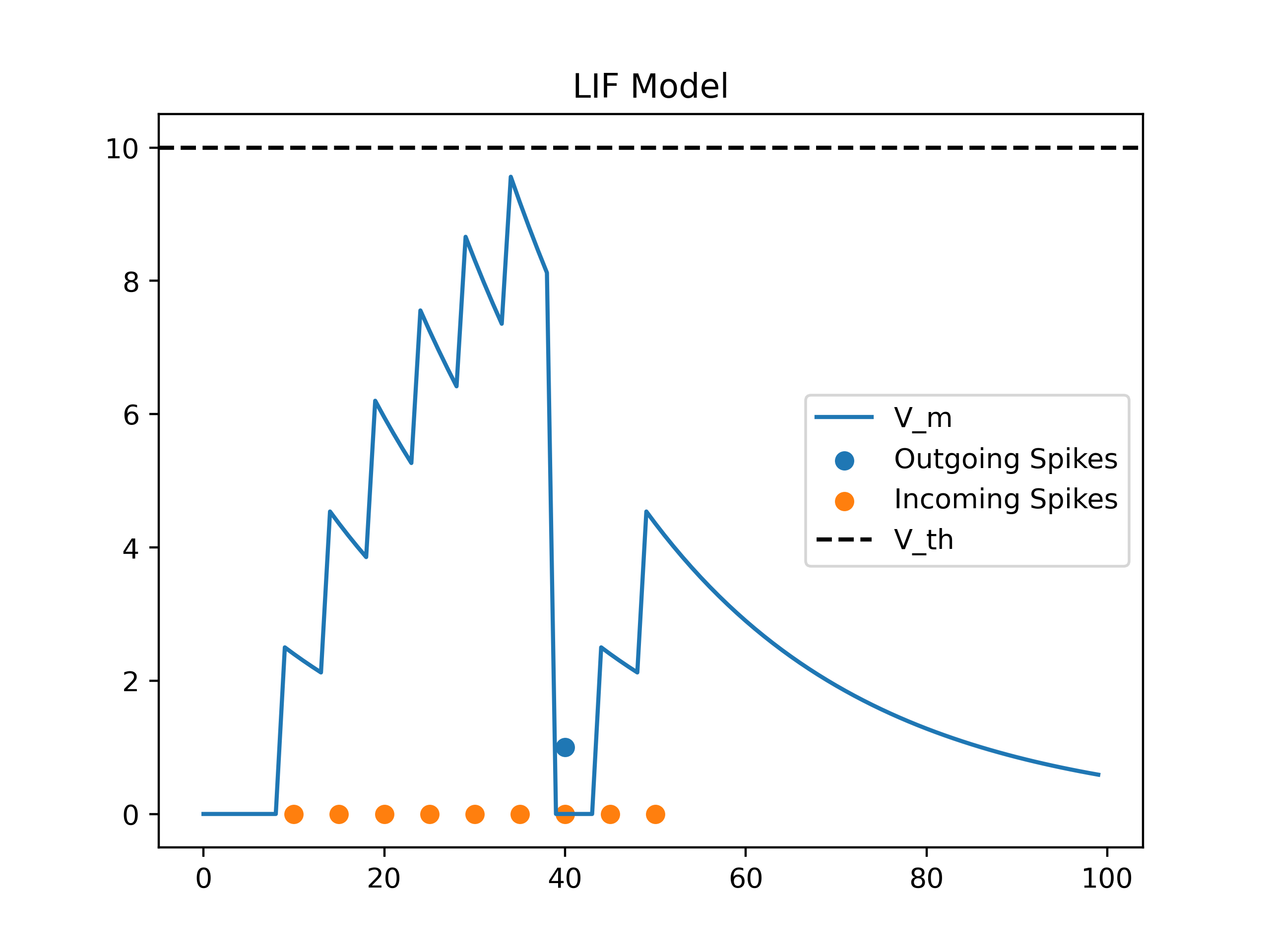
Notice that it seems as if the voltage never quite reaches the threshold value, this is because the incoming pulses are instantaneous and the pulse triggering an outgoing spike arrives in the same timestep the voltage is detected. More advanced models make this behavior smoother.
Discussion
Change the code to accept a non zero resting voltage
What happens to the neuron’s response if you change the value of \(tau\)?
What happens if the incoming synapses have a negative value?
More advanced models
The very simple LIF model exhibits some obvious defects, which are improved upon by other models:
In the current model, the effect of spikes is instantaneous and only lasts one timestep, which is unrealistic. Post-synaptic current (PSC) models introduce an extra differential equation for the synaptic current, which now also decays exponentially with time (or using other functional forms, such as the alpha model) instead of vanishing immediately. These models also usually include a refractory period, where the voltage of the neuron cannot be changed for a period of time after spiking.
Biological neurons are not able to spike constantly at the same rate, and go through a hardening period if repeatedly stimulated in a short period of time. Models such as the Izhikevich introduce more differential equations into the neuron model that can simulate complex effects such as ringing and sensitization.
The See Also section includes links to examples of some of these advanced models, and how to derive them and implement them in code. The following image shows the behavior of a PSC model:
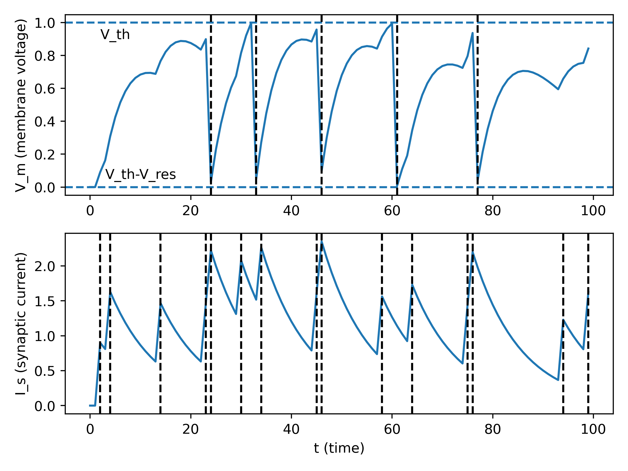
Notice that the increases in voltage when receiving a spike are much smoother, and that we also have to track the synaptic current dynamics.
Conclusion
Keypoints
The simplest LIF model can be implemented with a handful of lines of code
The model requires a number of parameters to be provided to be fully defined
This model can still exhibit quite complex behavior