Basics of PyNN

PyNN is a Python library that fucntions as an API to various neuromorphic computing simulators and hardware platforms. You can implement a spiking network in PyNN, and then use any of the other simulators as a backend to run the same network. As such, it allows the end user to only learn one itnerface, and apply it to a number of different simulation platforms. This makes it easier to transfer models, perform benchmarks on an even playing field, and compare simulators.

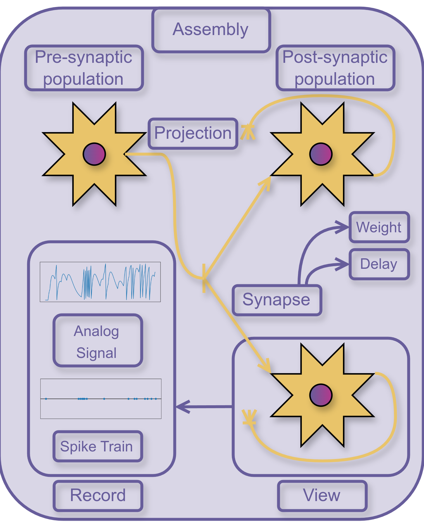
We will also use this opportunity to learn a number of concepts that are common across various NMC approaches. Here is a visual summary of the various PyNN and neuromorphic concepts:

Setting up a spiking neuron system

The first step is to import our desired backend simulator. There are some subtle differences between the various available simulators (such as minimum allowed synapse delay, maximum number of connections or spikes in a given timestep, etc.), but they are not relevant for our case studies. The idea of PyNN is that, in the end, the backend can be changed without needing to refactor the simulation we actually want to run.

# Boilerplate imports
import pyNN as pynn
import pyNN.neuron as sim #We'll be using Neuron as the backend
sim.setup(timestep=0.1) #ms, should be called at the very beginnin of the script to initialize PyNN correctly

/usr/local/lib/python3.13/site-packages/pyNN/neuron/__init__.py:14: UserWarning: mpi4py not available
  warnings.warn("mpi4py not available")

Warning: no DISPLAY environment variable.
--No graphics will be displayed.

0

Setting up the input to the network

The LIF neuron model is designed to stay at rest nif no stimulation is provided, and to return to the resting stage/voltage if not being actively driven. This applies to most neuron models. This means, if our simulation only contains standard neuron models, nothing will happen when we run it. Stimuli of some sort are required as “inputs” to the network. These can be, for example, signals from a different neuron network, or data that has been encoded in some way for signal processing or AI/ML tasks. It is also common to use arbitrary spiking sources. Two basic types exist:

• A spike train source, which spikes at specific, user provided timesteps. This can be used to encode specific incoming signals, or to drive the network in a specific, repeatable way.

• A Poisson source, that generates outgoing spikes at random following a statistical Poisson process. This is a more “natural” spike source and can be used to simulate, for example, background signal noise, or to drive a network stochastically. (NOTE: With careful usage of PyNN’s random number generator, the results of a Poisson source can be replicated consistently every simulation. The same applies for other RNG driven PyNN functions.)

We can set up a a spike train source as follows. Notice we are free to determine the incoming spikes array ourselves, which could then be specific times, something we generate at random, or following some sort of mathematical formula. Spike times are given as milliseconds since the beginning of the simulation. The strength of the spike source is defined by the synapse model chosen to connect it to the neuron population, which we will do later.

nspike=5
spikes=[1, 5, 10]
spike_source = sim.Population(nspike, 
            sim.SpikeSourceArray(spike_times=spikes)) #ms

For a Poisson source, the process is similar, but instead of providing specific spiking times, we need to provide an average spiking rate.

A note about units: There are various default units in use for neuromorphic simulations. For time, the usual unit is milliseconds. For rates such as the one in the Poisson source, the unit is Hz. Notice that this is 1/s, so if we want the source to spike, on average, once per timestep, we need a rate of around 1000 Hz. Question: What is the standard spiking rate range for biological neurons?

npoisson=5
noise_source = sim.Population(npoisson, 
            sim.SpikeSourcePoisson(rate=100)) #Hz

Setting up a neuron model

Neuron models are set up in a similar way as the spiking sources (in fact, they are similar objects in PyNN’s codebase). We need to provide the parameters for our model (pay attention to the units!), and add them to a population.

nneurons=5
# LIF Neuron Model
IF_params={
        'cm'         :   1.0, # nF, relationship between I and V, default 1.0; V = q/C, higher values mean less excitable neurons
        'i_offset'   :   0.0, # nA, current offset
        'tau_m'      :  20.0, # ms, membrane voltage decay, default 20.0
        'tau_refrac' :   0.1, # ms, refractory period, default 0.1
        'v_reset'    : -65.0, # mV, reset Vmembrane after triggering a spike, default -65.0
        'v_rest'     : -65.0, # mV, rest/initial Vmembrane, default -65.0
        'v_thresh'   : -45.0, # mV, threshold V for triggering a spike, default -50.0
        }
model   = sim.IF_curr_alpha(**IF_params)
pop = sim.Population(nneurons, model)

In many cases, we might want to generate neurons with a range of parameters instead of them all being clones of each other. This more accurately approximates a realistic biological situation, and can make your model/simulation more robust to changes in setup (otherwise, your solution might function only for a very specific set of parameters). PyNN provides functions for this. They can be used for the parameters of the nueron model, synapse parameters, etc.

Note: Be careful if you use the normal/Gaussian distribution, since it is unbounded. it might generate extreme values that might not make sense for your simulation, for example, negative parameters when only positive values should be allowed. There are bounded versions of the normal distribution available to avoid these complications.

rd = sim.RandomDistribution('uniform', (-55, -45))
IF_params={
        'v_thresh'   : rd, # mV, threshold V for triggering a spike, default -50.0
        }
model   = sim.IF_curr_alpha(**IF_params) # Set the spiking threshold, leaving all other parameters as default
pop_rd = sim.Population(nneurons, model)

Projections and Synapses: Connecting our populations

A “projection” is the process of setting up the connections between a pre- and post- synaptic population. It consist on a rule for connectiong both populations, and a synapse model. Various connecting rules exist:

• All to all (can be useful for optimization problems and ML, but computationally expensive)

• One to one (both populations same size)

• Fixed probability (neurons between both populations are connected at random with a given probability)

• Divergent/fan-out and convergent/fan-in

• Distance dependent (it is possible to introduce positions to a population, and use the geometric arrangement of the neurons to determine connection probability as well as other factors such as synapse delays, mimicing real network behaviors)

• User provided list (for systems where connections are already known, such as fully mapped small organisms with complete connectomes)

• Connection set algebra

• User-defined algorithm

Note that projections, by default, are uni-directional! If we want spikes to flow in the other direction, we have to explicitly set this up with another projection step.

As for synapse models, they can be as complex as the various available neuron models. The simplest synapse model has just two parameters:

• A weight: The strength of the connection between the neurons. Equivalent to the weight parameters in an artifical neuron network model.

• In some code libraries, the sign of the weight defines if it’s excitatory or inhibitory. In PyNN, this is defined by the “receptor_type” parameter.

• A delay: . This introduces a time component to the model of our system. Note that some simulators can have problems with a delay of 0 (that is, instantaneous spikes).

In more advanced simulations, the projection can be dynamic: which connections are present in the network and their strength is allowed to change as the simualtion progresses. This more closely reproduces behaviours in biological neuron networks such as learning.

synapse = sim.StaticSynapse(weight=15, delay=0)
sim.Projection(noise_source, pop, #pre-pop, post-pop
              connector=sim.OneToOneConnector(), #connection rule
              synapse_type=synapse,
              receptor_type="excitatory")

Projection("population1→population2")

Advanced: On Populations, Views, and Assemblies

PyNN provides different “containers” to manipulate and organize the neurons present in the simulation, which can be particularly useful as simulations grow in size and complexity.

The basic container is the population, which we have been using until now. We can obtain information about a population:

print(pop)
print(len(pop))

Population(5, IF_curr_alpha(<parameters>), structure=Line(dx=1.0, x0=0.0, y=0.0, z=0.0), label='population2')
5

and use the “dir” Python construct to see all the methods and properties available in it:

print(dir(pop))

['__add__', '__class__', '__delattr__', '__dict__', '__dir__', '__doc__', '__eq__', '__firstlineno__', '__format__', '__ge__', '__getattribute__', '__getitem__', '__getstate__', '__gt__', '__hash__', '__init__', '__init_subclass__', '__iter__', '__le__', '__len__', '__lt__', '__module__', '__ne__', '__new__', '__reduce__', '__reduce_ex__', '__repr__', '__setattr__', '__sizeof__', '__static_attributes__', '__str__', '__subclasshook__', '__weakref__', '_assembly_class', '_create_cells', '_get_cell_initial_value', '_get_cell_position', '_get_native_parameters', '_get_parameters', '_get_positions', '_get_structure', '_get_view', '_is_sorted', '_mask_local', '_nPop', '_native_rset', '_positions', '_record_filter', '_recorder_class', '_set_cell_initial_value', '_set_cell_position', '_set_initial_value_array', '_set_parameters', '_set_positions', '_set_structure', '_simulator', '_structure', 'all', 'all_cells', 'annotate', 'annotations', 'can_record', 'celltype', 'conductance_based', 'describe', 'find_units', 'first_id', 'get', 'getSpikes', 'get_data', 'get_gsyn', 'get_spike_counts', 'get_v', 'id_to_index', 'id_to_local_index', 'initial_values', 'initialize', 'inject', 'injectable', 'is_local', 'label', 'last_id', 'local_cells', 'local_size', 'meanSpikeCount', 'mean_spike_count', 'nearest', 'position_generator', 'positions', 'printSpikes', 'print_gsyn', 'print_v', 'receptor_types', 'record', 'record_gsyn', 'record_v', 'recorder', 'rset', 'sample', 'save_positions', 'set', 'size', 'structure', 'tset', 'write_data']

A view is a subset of a population. It can be generated in a number of ways, for example by slicing a population object using normal Python array notation. Views are useful for concentrating on a subset of a large population, for example sampling some neurons at random, or for setting up more complex projections.

Views and populations share most operations and methods. Changes to a view will reflect in the original population object, and vice-versa. They can be nested, that is, you can generate new views from other views.

print(pop[1:3])

PopulationView(parent=Population(5, IF_curr_alpha(<parameters>), structure=Line(dx=1.0, x0=0.0, y=0.0, z=0.0), label='population2'), selector=slice(1, 3, None), label="view of 'population2' with size 2")

Finally, assemblies are heterogeneous groupings of neurons. The neurons can belong to different populations or views, and even have different neuron models. Once again, these are useful for sampling or for setting up complex projections, or for creating populations of mixed neuron types.

my_assembly=spike_source+pop[1:3]
print(my_assembly)

Assembly(*[Population(5, SpikeSourceArray(<parameters>), structure=Line(dx=1.0, x0=0.0, y=0.0, z=0.0), label='population0'), PopulationView(parent=Population(5, IF_curr_alpha(<parameters>), structure=Line(dx=1.0, x0=0.0, y=0.0, z=0.0), label='population2'), selector=slice(1, 3, None), label="view of 'population2' with size 2")], label='assembly0')

Recording data

For the simpler spiking neuron simulations, we can extract two types of data:

• spike train: The outgoing spikes generated by a neuron. Note that if a neuron is being inhibited, it will not generate outgoing spikes, but its behavior might still be of interest. You will need to check the incoming spikes in this case, or the neuron’s internal voltage.

• analog signals: Usually voltage, but also current for models that care about it.

In particular, voltage signals can generate a large amount of data (one value per neuron per simulation timestep), so by default no data is recorded to avoid generating huge amounts of results. All data has to be explicitly recorded!. If you forgot to record the data for particular neurons of interest, you will need to rerun your simulation.

The record method can be set at the level of a population (or view, or assembly). Remember to do this before starting the simulation!

#Population.record(variables, to_file=None, sampling_interval=None)
# - sampling interval in ms; by default, every ms/timestep
# - variables: what exactly can be recorded is defined by each neuron model

pop.record(["spikes", "v"])

Running the simulation

runtime=100 #ms
sim.run(runtime)

99.99999999999646

Visualizing Results

The data recorded by PyNN is retreived in a Neo object, a common format for neurophisiological data. It can be somewhat tricky to handle, but in the end it is just NumPy arrays with extra structure.

The data is divided first ino segments, one per time the sim.reset operation was performed (in our case, only one segment). Each segment then contains a SpikeTrain and AnalogSignal object, depending on what was recorded. These also carry metadata such as units and sampling rate.

For spike trains, there will be one array per neuron in the originally recorded population (or view or assembly). The situation for analog signals is more complicated: there will be one “channel” per analog value recorded, and then as many arrays within each channel as sampling points. The length of each of these arrays is equal to the number of neurons sampled. That is, each array gives all the voltages (or other analog signal) of all the recorded neurons at a given timestep. This structure makes it a bit harder to reconstruct for data post-processing. The sampled timesteps are also stored.

The data hierarchy thus looks something like this

record
\-segment one
  \-spike train
    \- spike trains for first neuron
    \- spike trains for second neuron
    \- (...)
    \- spike trains for last neuron
  \-analog signal
    \-V
      \- voltages at first sampled timestep for all neurons
      \- voltages at second sampled timestep for all neurons
      \- (...)
      \- voltages at last sampled timestep for all neurons
      \-sampled times
    \-I
      \- (...)
\-segment two

# Extract and print the data
data=pop.get_data()
data.segments[0]

Segment with [<AnalogSignal(array([[-65.        , -65.        , -65.        , -65.        ,
        -65.        ],
       [-65.        , -65.        , -65.        , -65.        ,
        -65.        ],
       [-65.        , -65.        , -65.        , -65.        ,
        -65.        ],
       ...,
       [-63.93166755, -49.99815823, -50.75376686, -60.26722006,
        -58.07526391],
       [-63.92826188, -49.21850241, -50.82206369, -60.29076623,
        -56.63861896],
       [-63.92628224, -48.54064438, -50.89044455, -60.31419525,
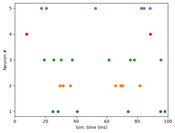
        -55.27162694]], shape=(1001, 5)) * mV, [0.0 ms, 100.1 ms], sampling rate: 10.0 1/ms)>] analogsignals, [<SpikeTrain(array([24.8, 28.2, 40.6, 73.9, 95.1, 97.9]) * ms, [0.0 ms, 99.99999999999646 ms])>, <SpikeTrain(array([29.4, 31.5, 36.3, 65.6, 69.2, 70.3, 81.7]) * ms, [0.0 ms, 99.99999999999646 ms])>, <SpikeTrain(array([19.2, 25.3, 30.2, 37.5, 61.5, 75.4, 78. , 95.3]) * ms, [0.0 ms, 99.99999999999646 ms])>, <SpikeTrain(array([ 7.7, 88.4]) * ms, [0.0 ms, 99.99999999999646 ms])>, <SpikeTrain(array([17.3, 20.6, 52.5, 82.7, 84.3, 88.3]) * ms, [0.0 ms, 99.99999999999646 ms])>] spiketrains
name: 'segment000'
description: 'Population "population2"\n    Structure   : Line\n    Local cells : 5\n    Cell type   : IF_curr_alpha\n    ID range    : 10-14\n    First cell on this node:\n      ID: 10\n      {}'
# analogsignals (N=[<AnalogSignal(array([[-65.        , -65.        , -65.        , -65.        ,
        -65.        ],
       [-65.        , -65.        , -65.        , -65.        ,
        -65.        ],
       [-65.        , -65.        , -65.        , -65.        ,
        -65.        ],
       ...,
       [-63.93166755, -49.99815823, -50.75376686, -60.26722006,
        -58.07526391],
       [-63.92826188, -49.21850241, -50.82206369, -60.29076623,
        -56.63861896],
       [-63.92628224, -48.54064438, -50.89044455, -60.31419525,
        -55.27162694]], shape=(1001, 5)) * mV, [0.0 ms, 100.1 ms], sampling rate: 10.0 1/ms)>])
0: AnalogSignal with 5 channels of length 1001; units mV; datatype float64
   name: 'v'
   annotations: {'channel_ids': array([10, 11, 12, 13, 14]),
     'source_population': 'population2'}
   sampling rate: 10.0 1/ms
   time: 0.0 ms to 100.1 ms

segdata=data.segments[0] #since there is only one segment, we can abbreviate
segdata.spiketrains[0] #spike train for the first neuron in our population

SpikeTrain containing 6 spikes; units ms; datatype float64 
annotations: {'source_population': 'population2',
  'channel_id': 10,
  'source_index': 0}
time: 0.0 ms to 99.99999999999646 ms

# Extract V data for all neurons
segdata.analogsignals[0]

AnalogSignal with 5 channels of length 1001; units mV; datatype float64
name: 'v'
annotations: {'channel_ids': array([10, 11, 12, 13, 14]),
  'source_population': 'population2'}
sampling rate: 10.0 1/ms
time: 0.0 ms to 100.1 ms

# Extract V data for one neuron
vdata=segdata.analogsignals[0]
vdata[0] # V data at first sampled timestep for all neurons

array([-65., -65., -65., -65., -65.]) * mV

len(vdata) # we can easily check that there are a lot of data points, since we sampled at every timestep of the simulation

1001

We can recover the sampled timesteps, which is useful for plotting purposes:

vdata.times

array([  0. ,   0.1,   0.2, ...,  99.8,  99.9, 100. ], shape=(1001,)) * ms

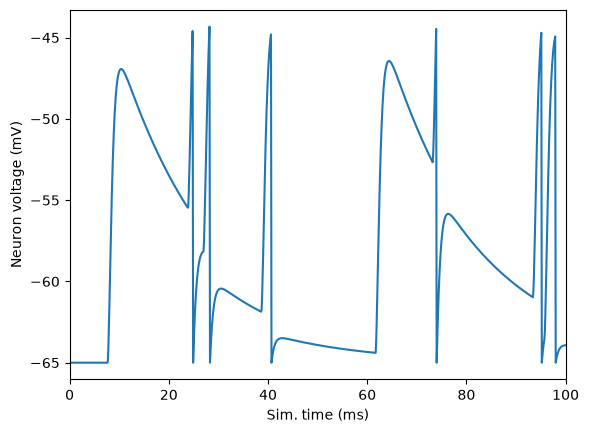
We can easily plot this data with matplotlib:

import matplotlib.pyplot as plt

# Neuron voltage for first recorded neuron
# Some tricky slicing is needed for the V data, there are multiple ways of doing this
neuron_index=0
plt.plot(vdata.times, vdata[:, neuron_index])
plt.xlabel("Sim. time (ms)")
plt.xlim(0.0, runtime)
plt.ylabel("Neuron voltage (mV)")
plt.show()

# Spike train for all neurons
# The data in this one is easier to process, but some extra steps are required to make the plot look better
spikes=segdata.spiketrains
for neuron_index, spike_data in enumerate(spikes): #go through each neuron's data
    scatter_pos=[neuron_index+1]*len(spike_data)
    plt.scatter(spike_data, scatter_pos)
plt.xlim([0.0, runtime]) # display time axis until end of simulation
plt.xlabel("Sim. time (ms)")
plt.yticks(range(1, len(spikes)+1)) # 1,2,3, etc. for Y axis, there are other ways of achieving this
plt.ylabel("Neuron #")
plt.show()

Optional tasks

• Does the voltage trace and spike train for your chosen neuron match? Can you plot one on top of the other?

• Record and plot the spikes of the Poisson sources. How do they behave? What happens if you increase or decrease their rate?