Introduction to neuromorphic computing concepts: Map Coloring algorithm
Introduction 
The classic problem of coloring a map in such a way that no adjacent regions share a color is a nice and simple introduction to constraint solving utilizing spiking neuron networks, and to common tricks and techniques that can be used in neuromorphic computing. It is also a simplified version of more complex graph optimization problems. For example, some small modifications can generate a network capable of coloring an arbitrary graph, or of solving the well-known puzzle Sudoku. This problem is just a subset of other, more complex graph based problems, and as such it is worth the effort to understand it.
This tutorial takes place after a basic PyNN introduction, so you should already know the basics of setting up neuron populations, connecting them with projections, accessing their data with views, etc.
Boilerplate code and imports
We need to import PyNN and set our chosen backend simulator. Here we will use Neuron, which is a bit simpler.
import numpy as np
import matplotlib.pyplot as plt
import pyNN as pynn
from pyNN.utility import get_simulator
import pyNN as pynn
from pyNN.utility import get_simulator
backend="neuron"
if backend == "nest":
    import pyNN.nest as sim
elif backend == "neuron":
    import pyNN.neuron as sim
else:
    print("Wrong backend selected")
    exit()
sim.setup()
/usr/local/lib/python3.13/site-packages/pyNN/neuron/__init__.py:14: UserWarning: mpi4py not available
  warnings.warn("mpi4py not available")
Warning: no DISPLAY environment variable.
--No graphics will be displayed.
NEURON mechanisms not found in /usr/local/lib/python3.13/site-packages/pyNN/neuron/nmodl.
0
Tricks in constraint optimization 
One hot encoding 
One hot encoding is a pretty common trick, also utilized in various machine learning techniques. It is used when we want to have an object representing a category (instead of a continuous value), where only one version of that category is possible. In our case, only one color should be possible for each location in our map. This can be achieved by the following configuration for each map location:
One neuron per possible color in our problem
Those neurons are connected to each other in an all-to-all configuration, with inhibitory synapses
The last consideration ensures that whenever one neuron is spiking, it will tend to shut off all the other ones. Do note that this is not a hard constraint: due to the way spiking neurons work, it is still possible for many neurons to spike if they are driven hard enough by external stimulation. But on average the system will tend to only have one spiking neuron at a time. This is a common behaviour in neuromorphic computing, there are no hard constraints!
To test this trick:
a) Set up a LIF neuron population of ncolors size
ncolors=5
# LIF Neuron Model
IF_params={
        'cm'         :   1.0, # nF, relationship between I and V, default 1.0; V = q/C, higher values mean less excitable neurons
        'i_offset'   :   0.0, # nA,
        'tau_m'      :  20.0, # ms, membrane voltage decay, default 20.0
        'tau_refrac' :   0.1, # ms, refractory period?, default 0.1
        'v_reset'    : -65.0, # mV, reset Vmembrane after triggering a spike, default -65.0
        'v_rest'     : -65.0, # mV, rest/initial Vmembrane, default -65.0
        'v_thresh'   : -45.0, # mV, threshold V for triggering a spike, default -50.0
        }
model   = sim.IF_curr_alpha(**IF_params)

pop = sim.Population(ncolors, model)
b) Feed the network with some random Poisson source noise, so all the neurons are driven at random. What would happen if you tried to run the simulation without the noise source?
## Poisson noise
delay=0.0
noise_source = sim.Population(ncolors,
            sim.SpikeSourcePoisson(rate=100, start=0.0))
synapse = sim.StaticSynapse(weight=15, delay=delay)
sim.Projection(noise_source, pop,
              connector=sim.OneToOneConnector(),
              synapse_type=synapse,
              receptor_type="excitatory")
Projection("population1→population0")
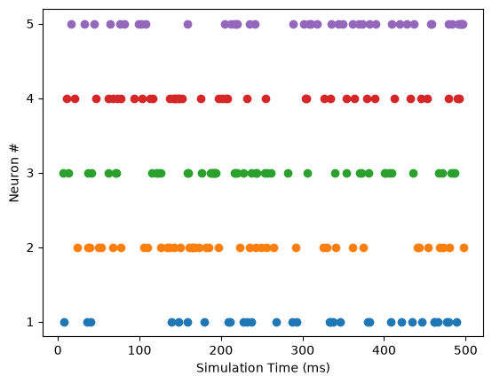
c) Run the simulation, and plot the spike trains for all the networks (don’t forget to set up the necessary recordings for this!). The cod for plotting the spike trains of a population is provided, or you can implement your own. How do the neurons behave?
NOTE: If you want to restart your simulation, you can use sim.reset(); but you might also have to set it up again from the beginning or it might accumulate the wrong objects! You might want to use the “Restart kernel and run up to selected cell” option in Jupyter.
# Recording
pop.record(["spikes", "v"])

runtime=500 #ms
sim.reset()
sim.run(runtime)
500.0000000000794
def plot_spiketrain(neuron_pop):
    data=neuron_pop.get_data()
    # Plotting
    plt.figure()
    for ni in range(0,len(neuron_pop)): # Loop through population
        spt=data.segments[0].spiketrains[ni]
        # for a scatter plot we need a Y position, we can assign each one the neuron number, this also stands in for the neuron color
        # this vector needs to be the same size as the spiketrain,
        ypos=[ni+1]*len(spt)
        plt.scatter(spt, ypos, color="C{}".format(ni)) #use matplotlib's color wheel for nice colors
    plt.ylabel("Neuron #")
    plt.xlabel("Simulation Time (ms)")
    # Set Y-Axis to only tick at integer values for aesthetic purposes
    plt.yticks(range(1,len(neuron_pop)+1))
    plt.show()

data=pop.get_data()
# Our simulation will only have one segment, and as many spiketrains as there are neurons in this population
print(data.segments[0].spiketrains[0])
print(data.segments[0].spiketrains[1])

plot_spiketrain(pop)
[  7.1  36.1  39.8 139.2 147.7 159.1 179.8 209.  211.3 227.9 231.6 237.1
 267.8 287.  293.  332.7 334.2 337.1 346.2 379.9 381.9 408.7 421.8 434.
 446.6 461.1 462.  465.6 476.9 479.4 488.3] ms
[ 23.5  37.2  38.9  49.6  53.4  66.9  76.6 105.9 109.4 125.9 134.2 137.5
 142.6 150.5 161.4 163.8 165.1 167.1 172.6 181.7 185.3 197.3 223.5 235.2
 243.  249.7 255.5 264.5 291.7 325.7 330.1 340.3 361.2 374.2 440.8 443.
 454.  467.8 472.4 480.2 497.1] ms
d) Connect the neurons all-to-all with a projection, using an inhibtory synapse weight (and no delay). Compare the new behaviour with the previous one. Have we achieved a one-hot setup?
Hint 1: You can project a population onto itself!
Hint 2: Look into the AllToAll connector
Hint 3: Do we want to allow neurons to inhibit themselves? How can you regulate this in the AllToAll connector?
# One-hot constraint implementation
delay=0
synapse = sim.StaticSynapse(weight=-20, delay=delay)
sim.Projection(pop, pop,
              connector=sim.AllToAllConnector(allow_self_connections=False),
              synapse_type=synapse,
              receptor_type="inhibitory")
Projection("population0→population0")
# Recording and running
pop.record(["spikes", "v"])

runtime=500 #ms
sim.run(runtime)
999.9999999996382
plot_spiketrain(pop) # notice how we go from random spiking, to random spiking but only 1 neuron at a time, to consistent spiking of a sinlge neuron at a time
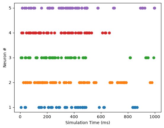
e) Play around wtih the value of the Poisson noise source strength. What happens if this is very strong compared with the inhibitory synapse strength?
Self excitation
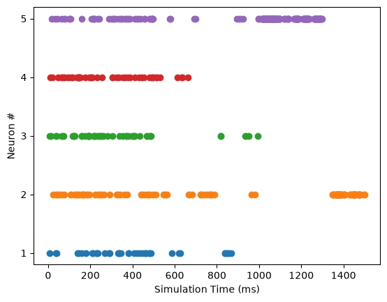
From the previous section, you might have noticed that neurons in the network will spike at random due to external Poisson source, and stop others from spiking for a small period of time, but eventually shut down and let another neuron take over. This is useful, but does not allow our network to reach a “consensus”. We want a situation where a neuron that has spiked once will continue to spike. When neurons spike, their voltage is lowered, and as such they lose “energy” and are not likely to spike again unless stimulated further.
To achieve this configuration, we can connect each neuron to itself with an excitatory connection! This means that once a neuron has spiked, it will reinforce itself, and be ready to spike or close to spiking again in the next time step. One needs to be careful with the values here: if the self stimulation is too strong, neurons will ignore external considerations and the network will become stuck. If it’s too weak, the neurons will be too sensitive and will not reach a consensus.
a) Continue from the network considered in the previous point. Add an excitatory connection to every neuron with itself (this is possible with a single projection command).
Hint 1: As before, you can project a population into itself.
Hint 2: Look into the OneToOne connector. Does it allow self connections?
# Self excitation
delay=0
synapse = sim.StaticSynapse(weight=15, delay=delay)
sim.Projection(pop, pop,
              connector=sim.OneToOneConnector(),
              synapse_type=synapse,
              receptor_type="excitatory")
Projection("population0→population0")
b) Simulate the network and plot the spike trains. What do you notice in comparison with before? Do you obtain more consistent spiking periods? What happens if you change the strength of the self-synapse?
sim.run(runtime)
1499.9999999991835
plot_spiketrain(pop)
Setting up constraints
Until now, we have set up a small network that can exhibit consistent one-hot encoding behaviour. Our next step is to set up multiple sub-networks (each representing one location in our map or one edge in our graph), and connecting them with a constraint.
The constraints in this situation are that:
For each location, only one color is possible (we have already solved this!)
Across connected locations, colors should not be shared
How can we achieve this final condition? Each location has one neuron standing in for a color (arbitrarily, we can say the first neuron in each population is red, the second green, etc.). What happens if you connect equivalent neurons across populations with an inhibitory synapse?
a) Create as many populations as there are colors. For example, let’s try 3 populations/locations for 3 colors.
# Start a new simulation
import pyNN.neuron as sim
sim.setup()

# Generate populations
ncolors=2
npops=8#ncolors
pops=[]
for ni in range(npops):
    newpop = sim.Population(ncolors, model, label=ni)
    pops.append(newpop)

## Poisson noise
delay=0.0
for pop in pops:
    # Need to generate a new Poisson source for each pop or they will all get the same exact noise
    noise_source = sim.Population(ncolors,
            sim.SpikeSourcePoisson(rate=50, start=0.0))
    synapse = sim.StaticSynapse(weight=20, delay=delay)
    sim.Projection(noise_source, pop,
              connector=sim.OneToOneConnector(),
              synapse_type=synapse,
              receptor_type="excitatory")

# One-hot constraint
delay=0
synapse = sim.StaticSynapse(weight=-20, delay=delay)
for pop in pops:
    sim.Projection(pop, pop,
              connector=sim.AllToAllConnector(allow_self_connections=False),
              synapse_type=synapse,
              receptor_type="inhibitory")

# Self excitation
delay=0
synapse = sim.StaticSynapse(weight=15, delay=delay)
for pop in pops:
    sim.Projection(pop, pop,
              connector=sim.OneToOneConnector(),
              synapse_type=synapse,
              receptor_type="excitatory")

# Recording
for pop in pops:
    pop.record(["spikes", "v"])
b) Connect equivalent neurons with inhibitory synapses. For the 3 location case, imagine our locations are all adjacent to each other. Connect neuron 1 in population A to neuron 1 in population B and neuron 1 in population C, neuron 2 to all other neuron 2’s, etc. Be efficient here, you probably want a nice loop.
NOTE: Be very careful here, projections are by default unidirectional! Should the connection in this case be uni- or bi-directional? Is there an option for bidirectional connections in PyNN? Or do you have to do these manually in both directions? Avoid double counting connections! This is the most complicated setup we will do.
# Cross population constraints
synapse = sim.StaticSynapse(weight=-10, delay=delay)
## Forwards
for ipop, pop in enumerate(pops):
    pre_pop=pop
    if (ipop+1) != len(pops): # Check if we are wrapping around at the last population, which should connect last-> first
        post_pop=pops[ipop+1]
    else:
        post_pop=pops[0]
    sim.Projection(pre_pop, post_pop,
              connector=sim.OneToOneConnector(),
              synapse_type=synapse,
              receptor_type="inhibitory")
## Backwards
for ipop, pop in enumerate(pops):
    pre_pop=pops[ipop-1] #we don't need a special check here since [0-1]=[-1] which will return the last element of pops
    post_pop=pop
    sim.Projection(pre_pop, post_pop,
              connector=sim.OneToOneConnector(),
              synapse_type=synapse,
              receptor_type="inhibitory")
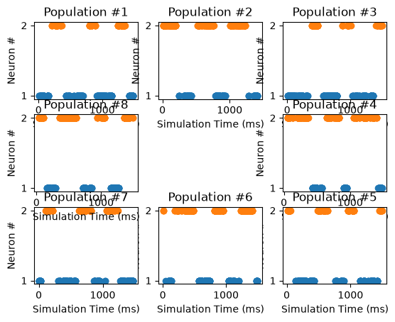
c) Run and plot your network. Play around with the value of the inhibitory cross-population connection.
runtime=1500 #ms
sim.run(runtime)
1499.9999999991835
# Helper to plot an 8 member ring into subplots in a 3X3 grid
# Pyplot:
#|1|2|3|
#|4|5|6|
#|7|8|9|
# We want:
#|0|1|2|
#|7|X|3|
#|6|5|4|
ring_plot_pos={0:1, 1:2, 2:3, 3:6, 4:9, 5:8, 6:7, 7:4}
def plot_spiketrain_multipops(neuron_pops):
    #data=neuron_pop.get_data()
    npops=len(neuron_pops)
    if npops != 8: # general case:
        ncols=npops
        nrows=1
    else:# Ring plot case
        ncols=3
        nrows=3
    # Plotting
    plt.figure()
    for ipop, pop in enumerate(pops): #for each pop
        if npops != 8: # general case:
            subplot_pos=ipop+1
        else: # Ring plot case
            subplot_pos=ring_plot_pos[ipop]
        plt.subplot(ncols, nrows, subplot_pos) #change to a new subplot
        data=pop.get_data()
        for ineuron,neuron in enumerate(pop): # then loop through each neuron in that population
            spt=data.segments[0].spiketrains[ineuron]
            # for a scatter plot we need a Y position, we can assign each one the neuron number, this also stands in for the neuron color
            # this vector needs to be the same size as the spiketrain,
            ypos=[ineuron+1]*len(spt)
            plt.scatter(spt, ypos, color="C{}".format(ineuron)) #use matplotlib's color wheel for nice colors
        plt.ylabel("Neuron #")
        plt.xlabel("Simulation Time (ms)")
        plt.title("Population #{}".format(ipop+1))
        # Set Y-Axis to only tick at integer values for aesthetic purposes
        plt.yticks(range(1,len(pop)+1))
    plt.show()

plot_spiketrain_multipops(pops)
Random Noise
In the previous sections we used a random external noise source to drive the network. Why? What happens if there is no excitation coming into the network(s)? Can LIF neurons spike by themselves, or do they always return to a resting state?
Note: If you’ve ever done molecular simulations or have some chemistry background or experience with optimization algorithms, you can think of the Poisson noise source as a temperature source that allows the system to explore different configurations, and injects energy into the system to allow it to climb over energy barriers. I find analogies to molecular simulations very useful when thinking about neuron networks.
a) Repeat your previous simulation, but change the strength of the Poisson source. What happens at the extremes, when it is too weak or too strong?
Clues
In some cases, you might want to pre-define parts of your network. That is, provide specific locations that should be pre-colored in a given way (let us call this a “clue”, since it makes deciphering the final state of your simulation easier). You could to this by treating those locations and neurons specially, but a more flexible way is to set up an external constantly spiking source that provides a consistent clue source.
a) Set up a clue population, which should be a constantly spiking source. Connect it to a one of the neurons in your network. Run your simulation and plot it. Is your clue taken into account? What happens if the clue source strength is changed?
Optional: Putting it all together: A map coloring network
Draw your network
If you’ve gone through the previous section, you probably realize we now have a lot of different components interacting. It is highly recommended you take pen and paper (or your favorite diagram making tool) and draw the main components of our algorithm and their inhibitory or excitatory connections. That would be:
one-hot encoding population, one per map location, connected ot each other with inhibitory synapses
self-exciting connections
random noise source
clue source
inhibitory conenctions across locations for equivalent neurons
Setting up our map (or graph)
Use a Numpy array or tensor, or a Python library for working with graphs, and set up your simulation.
Takeaways
Giving your simulation meaning
Notice that in our simulation, the meaning arises from the connections we set up for the different populations. Cocnepts such as one-hot encoding or constraints are imposed by us. The same applies to a simulation of nervous tissue: the identity of the different neuron populations arises from the models we assign to them, the parameters we provide them with, and the synapses we create.
Limitations and Performance
We have looked at very small networks. What do you consider the main limitation to the performance of our algorithm? How many neurons are needed per location and per possible color? What about the number of synapses?
Optimization and Global Minima
In this case we have a rather simple simulation. In more complex configurations, it will not always be possible to perfectly optimize and satisfy all constraints at the same time. In those cases, your network might be able to find a solution (a global minimum), but not necessarily the best solution (a global maximum).
Over and under defined problems
Similar to simple systems of equations, constraint problems can be over- or underdefined (wrong ratio of clues vs. constraints and known variables). It is well known that at least for a 2 dimensional map, 3 colors are enough to satisfy all the constraints of the map coloring problem (tho this might not necessarily be the case with an arbitrary graph where connections are not limited to those possible on a 2D surface). What happens if you set up your network with more than 3 colors? What happens if you use only 2? What happens if you provide a lot of clues, or contradicting clues?
Parameters in your network
Notice that in this case weare simulating arbitrary “neurons” without a direct biological analogue. As such, we don’t ahve reference parameters for the various configurable values in the simulation (all the LIF values, the strength of the Poisson source, the strength of the different constraint synapses). You will need to experiment to find the correct range of values that return a functioning simulation. Usually you need to take into account the parameters of the LIF model such as the resting voltage and the spiking threshold, and set the other values in relation to this. It might be useful to set them as a factor of these so they can be more easily adjusted.
Beyond: Extending to a Sudoku solving network
A network that can solve the classic Sudoku puzzle is very similar to the map coloring network. SOme differences of note:
We are dealing with numbers, isttead of colors (but in the end these are arbitrary)
All of the techniques considered in the map coloring example are still needed (one-hot encoding, external Poisson source, self-excitation, cross-constraints, and clues, which are of course even more important than in the map coloring case)
The cross population constraints are the biggest difference. In Sudoku, numbers cannot be repeated:
In a column
In a row
In a subsection of the puzzle
The best approach here is to use a numpy tensor to set up the board and one-hot encoding. Each slot in the tensor will contain a neuron object, and the connections built upon them will set up the SUdoku network. The trickiest part of the algorithm is setting up the subsection contraint (and handling the tensor and indexing and slicing notation in general). We highly recommend starting with a smaller 4X4 puzzle with the numnbers 1 through 4 instead of the larger, common 9X9 puzzle (tho if set up correctly the size can be changed on the fly).
As a final note, you can try to math it out, and you will see that the number of synapses required for setting up the constraints grows very quickly as the Sudoku size increases.